本文是三篇 TF 2.0 学习笔记合集（合并自原 Functions, not Sessions / Distributed training with TensorFlow / Notes for Distributed Tensorflow 2.0）。

1 Functions, not Sessions

（原文写于 2020-05-07）

doc link

1.1 Design Proposal

Basic idea: Python functions as Graphs

Where tf.function is a decorator that “defines a TensorFlow function”. A “TensorFlow function” defines a computation as a graph of TensorFlow operations, with named arguments and explicit return values.

1
2
3
4
5
6
7
8
9
10
11
12

import tensorflow as tf

@tf.function
def compute_z1(x, y):
  return tf.add(x, y)

@tf.function
def compute_z0(x):
  return compute_z1(x, tf.square(x))

z0 = compute_z0(2.)
z1 = compute_z1(2., 2.)

Having the Python function correspond to what the runtime will execute reduces conceptual complexity in translating between the two domains.

Referencing state: Variables, tables etc.

A function decorated Python function encapsulates a graph and its execution. The Python function may reference stateful objects (i.e., state backed by DT_RESOURCE tensors in the runtime, e.g., tf.Variable) by referencing the corresponding Python object, and these will be captured as implicit inputs to the function.

Comparing TensorFlow code today with how we propose it looks in 2.x:

1
2
3
4
5
6
7
8
9
10
11
12
13
14
15
16
17
18
19
20
21
22
23
24
25
26
27
28
29
30
31
32
33
34

# TF 1.x
W = tf.Variable(
  tf.glorot_uniform_initializer()(
    (10, 10)))
b = tf.Variable(tf.zeros(10))
c = tf.Variable(0)

x = tf.placeholder(tf.float32)
ctr = c.assign_add(1)
with tf.control_dependencies([ctr]):
  y = tf.matmul(x, W) + b
init =
  tf.global_variables_initializer()

with tf.Session() as sess:
  sess.run(init)
  print(sess.run(y,
  feed_dict={x: make_input_value()}))
  assert int(sess.run(c)) == 1

# TF 2.0
W = tf.Variable(
  tf.glorot_uniform_initializer()(
    (10, 10)))
b = tf.Variable(tf.zeros(10))
c = tf.Variable(0)

@tf.function
def f(x):
  c.assign_add(1)
  return tf.matmul(x, W) + b

print(f(make_input_value())
assert int(c) == 1

Worthy of note here - in TensorFlow 1.x, the memory underlying the variables W and b in the runtime lives for the lifetime of the Session - unrelated to the lifetime of the Python objects. In 2.x, the lifetime of the Python objects and the runtime state are tied together.

Control dependencies

In TensorFlow graphs today, control dependencies are sometimes needed to ensure correct evaluation order.

1
2
3
4
5
6
7
8
9
10
11
12
13
14
15
16
17
18
19
20
21

# TF 1.x
v = tf.Variable(1.0)
init_op = tf.global_variables_initializer()
assign_op = v.assign(2.0)
read = v.read_value()

with tf.Session() as sess:
  sess.run(init_op)
  val = sess.run(read)
  print(val) # Will print 1.0, the assign is ignored
  val = sess.run([read, assign_op])[0]
  print(val)   # Non-deterministically prints 1.0 or 2.0,

# TF2.0
v = tf.Variable(1.0)
@tf.function
def f():
  v.assign(2.0)
  return v.read_value()

print(f()) # Always prints 2.0.

Note that the intention here is to avoid observable differences from program order. For example:

1
2
3
4
5
6
7
8

a = tf.Variable(1.0)
b = tf.Variable(1.0)
@tf.function
def f():
  a.assign(2.0)
  b.assign(3.0)
  return a + b
print(f())

Will always print 5.0 since the assignments will occur before the read. However, there is no guaranteed ordering between the assignment of a and b (as any difference in that is not observable).

Functions that create state

1
2
3
4
5
6
7
8
9
10
11

v = None

@tf.function
def f(x):
  global v
  if v is None:
    v = tf.Variable(1.0)
  return tf.cast(x, tf.float32) + v

f(tf.constant(1, dtype=tf.float32)) # Creates the variable, returns 2.0
f(tf.constant(2, dtype=tf.int32))   # Reuses the variable, returns 3.0

1. State (like tf.Variable objects) are only created the first time the function f is called. If any variables are created in the first execution of f, then @tf.function will trace f again the second time it is invoked in order to record the behavior that will be used from then on.
2. The caller must make sure that any variable referenced by the function still exists whenever the function is evaluated. @tf.function itself will keep only weak references to these created variables.

Trace Caches

Since new graphs are traced when new input signatures are encountered, a function can encapsulate multiple graphs. For example, considering the following, there are two graphs created here:

1
2
3
4
5
6

@tf.function
def f(x):
  return tf.square(x)

f(tf.constant(1, dtype=tf.int32))
f(tf.constant(1.0, dtype=tf.float32))

Note the use of tf.constant to ensure that the argument is a Tensor. If the argument were a Python value, then additional graphs will be traced for each such value. For example, the following two calls will result in two additional graphs being traced:

1
2

f(1.0)
f(2.0)

Where arguments are not Tensors, the “value” of the argument is used to compute the trace_cache_key. For example:

1
2
3
4
5
6

@tf.function
def f(x, use_multiply):
  return tf.multiply(x, x) if use_multiply else tf.square(x)

f(tf.constant(2.0), True)
f(tf.constant(2.0), False)

will result in 2 graphs being created, since the two calls result in two different cache keys because the value of the Python object (the second argument) changes between the two.

Note that the “type” of Tensor inputs to the function also incorporates the shape. For example:

1
2
3
4
5
6
7
8
9

@tf.function
def f(x):
	return tf.add(x, 1.)

f(tf.constant([2.0]))
f(tf.constant([2.0, 3.0]))
f(tf.constant([[2.0]]))
f(tf.constant([3.0]))
f(tf.constant([4.0, 5.0]))

will result in 3 graphs being created.

The trace_cache_key also incorporates the “context” in which the call was made. For example:

1
2
3
4
5
6
7

@tf.function
def f(x): return tf.add(x, 1.)

with tf.device("/device:CPU:0"):
  f(tf.constant(2.0))
with tf.device("/device:GPU:0"):
  f(tf.constant(2.0))

Will create 2 graphs.

CAUTION: Too many traces

CAUTION: Mutable non-Tensor arguments

The trace_cache_key includes the Python object for non-Tensor arguments. Mutations of these arguments might not be detected. For example:

1
2
3
4
5
6
7
8
9
10
11
12

# non-Tensor object
class Params(object):
  multiply = True

p = Params()
@tf.function
def f(x, y):
  return tf.multiply(x, 2.) if y.multiply else tf.add(x, 2.)

f(3., p) # Returns 6.0
p.multiply = False
f(3., p)  # Mutations to `p` may not trigger a retrace, so might still return 6.0

Input Signatures

An “input signature” can be explicitly specified to control the trace_cache_key computation based on the type and shape of Tensor (and list of Tensor) arguments to f.

1
2
3
4
5
6
7
8
9
10
11
12
13
14

@tf.function(input_signature=((tf.float32, [None]))
def f(x):
	return tf.add(x, 1.)

f(tf.constant([2.0]))      # Returns [3.0]
f(tf.constant([2.0, 3.0])) # Matches the input signature as [None]
                           # matches the actual shape [2]
f(tf.constant([[2.0]]))    # Raises an error as the arguments don't match the
                           # input signature.
f(tf.constant([2], dtype=tf.int32)) # Raises an error as the dtype of the argument
                                    # does not match the input signature

# f is backed by a single Graph since the input signature specification allowed
# for the same graph to be used when the input shape is (1,) or (2,).

1. For a Tensor argument, it specifies a (dtype, shape pattern).
   • (tf.float32, [None]) means the argument must be a float32 vector (with any number of elements).
   • (tf.int32, []) means that the argument must be an int32 scalar.
2. For a list of Tensor objects, it specifies an optional list length and the signature for elements in the list (i.e., the dtype and shape pattern for all elements in the list).
3. For non-Tensor arguments: tf.PYTHON_VALUE

You can use the tf.TRACE_ON_NEW_VALUE to release the restriction of dtype:

1
2
3
4
5
6

@tf.function(input_signature=((tf.TRACE_ON_NEW_VALUE, [None]))
def f(x):
	return tf.square(x)

f(tf.constant([2.0])) # Returns 4.0
f(tf.constant([2, 2], dtype=tf.int32) # Returns [4, 4] after tracing a new graph

Classes

If a member function of a class does not create variables, it may be decorated with @tf.function and it will work:

1
2
3
4
5
6
7
8
9
10
11
12
13
14
15
16
17
18

class AnyShapeModel(object):
  def __init__(self):
    self.v = None

  @tf.function
  def increment(self, amount):
    if self.v is None:
      self.v = tf.Variable(tf.zeros_like(amount))
    self.v.assign_add(amount)

model1 = AnyShapeModel()
model1.increment(tf.constant(3))
assert int(model1.v) == 3
model1.increment(tf.constant(4))
assert int(model1.v) == 7
model2 = AnyShapeModel()
model2.increment(tf.constant([4, 5]))
assert model2.v.numpy() == [4, 5]

The semantics here are that each new instance is allowed to create variables in each @tf.function once.

function-ing Python control flow

If the function has data-dependent control flow then though the function will execute fine with eager execution enabled, function decorating it will fail. For example:

1
2
3
4
5
6
7
8
9
10
11
12

def f(x, y):
  if tf.equal(y, 0.0):
    return y
  return x / y

x = tf.constant(2.0)
y = tf.constant(2.0)

f(x, y) # Will be 1.0

df = tf.function(f)
df(x, y)  # Will raise an error complaining about the data-dependent control flow

To fix this, one would have to use the graph construction APIs for control flow (tf.cond, tf.while_loop):

1
2
3
4
5
6
7
8
9
10

def f(x, y):
  return tf.cond(tf.equal(y, 0.0), lambda: y, lambda: x/y)

x = tf.constant(2.0)
y = tf.constant(2.0)

f(x, y) # Will be 1.0

df = tf.function(f)
df(x, y)  # Will be 1.0

This situation can be improved with the help of autograph to allow expression of control flow in Python.

1
2

df = tf.function(autograph=True)(f)
f(x, y) # Will be 1.0

2 Distributed Training & Strategy

（原文写于 2020-05-09 / 2020-05-12，合并 Strategy 概念与使用）

参考：tf.distribute.Strategy guide

2.1 Parallelism

TensorFlow’s basic dataflow graph model can be used in a variety of ways for machine learning applications. However, some neural networks models are so large they cannot fit in memory of a single device (GPU). Google’s Neural Machine Translation system is an example of such a network.

Such models need to be split over many devices, carrying out the training in parallel on the devices. There are three method to train a model in parallel on the devices: Model parallelism, Data parallelism, and Model Computation Pipelining.

Model parallelism uses same data for every device but partitions the model among the devices. The graph is split as several sub-graphs, and assigns these sub-graphs to feasible devices to training. All devices use a same mini-batch to train.

Data parallelism uses the same model for every device, but train the model in each device using different training samples. Each device holds a entire model, but trains with partial samples from the mini-batch.

Model Computation Pipelining pipelines the computation of seveal same models within one device by running a small number of concurrent steps.

Model parallelism

Model parallel training, where different portions of the model computation are done on different computational devices simultaneously for the same batch of examples, as the following figure:

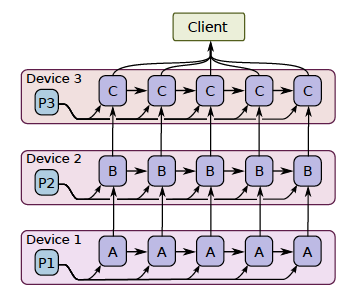
It is challenging to get good performance, because some layers may depend on previous layers which leads to a long waiting time. However, if a model has some components which can run in parallel, it can use this method to improve the efficiency.

Data parallelism

In modern deep learning, because the dataset is too big to be fit into the memory, we could only do stochastic gradient descent(SGD) for batches. The shortcoming of SGD is that the estimate of the gradients might not accurately represent the true gradients of using the full dataset. Therefore, it may take much longer to converge.

Data parallelism is a simple technique for speeding up SGD is to parallelize the computation of the gradient for a mini-batch across devices.

Each device will independently compute the loss the gradients of small batches, the final estimate of the gradients is the weighted average of the gradients calculated from all the small batches(require communication).

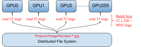
By using data parallelism, the model can train on a large batch size. For example, the folloing figure shows a typical data parallelism, distributing 32 different images to each of the 256 GPUs running a single model. Together, the total mini-batch size for an iteration is 8,092 images (32 x 256) (Facebook: Training ImageNet in 1 Hour).

Mathematically, data parallelism is valid because:

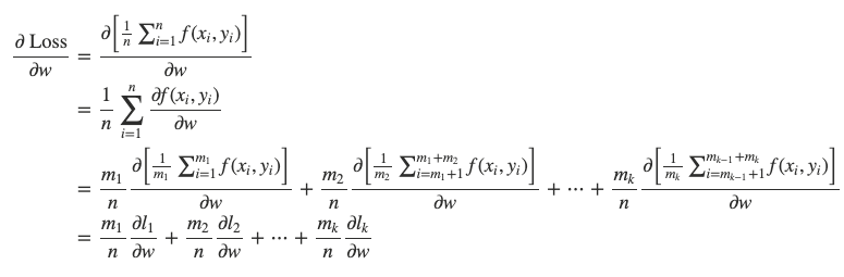
* m1+m2+⋯+mk=n.

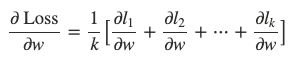
When m1=m2=⋯=mk=nk, we could further have:

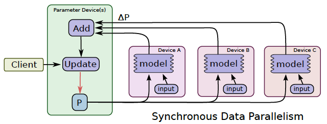
Synchronous vs asynchronous training

In synchronous training(as following figure), all of the devices train their local model using different parts of data from a single (large) mini-batch. They then communicate their locally calculated gradients (directly or indirectly) to all devices.

Only after all devices have successfully computed and sent their gradients is the model updated. The updated model is then sent to all nodes along with splits from the next mini-batch. That is, devices train on non-overlapping splits (subset) of the mini-batch.

In asynchronous training, no device waits for updates to the model from any other device. The devices can run independently and share results as peers, or communicate through one or more central servers known as “parameter” servers.

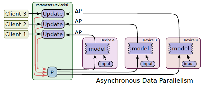
In synchronous training, the parameter servers compute the latest up-to-date version of the model, and send it back to devices. In asynchronous training, parameter servers send gradients to devices that locally compute the new model.

Model Computation Pipelining

Another common way to get better utilization for training deep neural networks is to pipeline the computation of the model within the same devices, by running a small number of concurrent steps within the same set of devices.

It is somewhat similar to asynchronous data parallelism, except that the parallelism occurs within the same device(s), rather than replicating the computation graph on different devices.

This allows “filling in the gaps” where computation of a single batch of examples might not be able to fully utilize the full parallelism on all devices at all times during a single step.

2.2 tf.distribute.Strategy types

tf.distribute.Strategy is a TensorFlow API to distribute training across multiple GPUs, multiple machines or TPUs. It intends to cover a number of use cases along different axes:

• synchronous vs asynchronous training (sync via all-reduce, async via parameter server),
• hardware platform (multi-GPU on one machine, multi-machine, Cloud TPUs).

MirroredStrategy

Supports synchronous distributed training on multiple GPUs on one machine. It creates one replica per GPU device. During training, one mini-batch is split into N parts and each part feeds one GPU.

Efficient all-reduce algorithms are used to communicate the variable updates across the devices. By default, it uses NVIDIA NCCL as the all-reduce implementation. tf.distribute.HierarchicalCopyAllReduce and tf.distribute.ReductionToOneDevice are two options other than tf.distribute.NcclAllReduce.

1
2
3
4
5
6

mirrored_strategy = tf.distribute.MirroredStrategy()
# or with explicit device list:
mirrored_strategy = tf.distribute.MirroredStrategy(devices=["/gpu:0", "/gpu:1"])
# or with custom all-reduce:
mirrored_strategy = tf.distribute.MirroredStrategy(
    cross_device_ops=tf.distribute.HierarchicalCopyAllReduce())

CentralStorageStrategy

Synchronous training as well. Variables are not mirrored, instead they are placed on the CPU and operations are replicated across all local GPUs. If there is only one GPU, all variables and operations will be placed on that GPU.

1

central_storage_strategy = tf.distribute.experimental.CentralStorageStrategy()

MultiWorkerMirroredStrategy

Very similar to MirroredStrategy, but implements synchronous distributed training across multiple workers, each with potentially multiple GPUs. Creates copies of all variables on each device across all workers.

It uses CollectiveOps as the multi-worker all-reduce communication method — a single op in the TensorFlow graph that automatically chooses an all-reduce algorithm in the TensorFlow runtime according to hardware, network topology and tensor sizes.

Two implementations of collective ops:

• CollectiveCommunication.RING — ring-based collectives using gRPC as the communication layer.
• CollectiveCommunication.NCCL — NVIDIA NCCL for all-reduce, ring algorithms for all-gather.

1
2

multiworker_strategy = tf.distribute.experimental.MultiWorkerMirroredStrategy(
    tf.distribute.experimental.CollectiveCommunication.NCCL)

TPUStrategy

Lets you run TensorFlow training on Tensor Processing Units (TPUs).

1
2
3
4

cluster_resolver = tf.distribute.cluster_resolver.TPUClusterResolver(tpu=tpu_address)
tf.config.experimental_connect_to_cluster(cluster_resolver)
tf.tpu.experimental.initialize_tpu_system(cluster_resolver)
tpu_strategy = tf.distribute.experimental.TPUStrategy(cluster_resolver)

ParameterServerStrategy

Supports parameter servers training on multiple machines. Some machines are designated as workers and some as parameter servers. Each variable of the model is placed on one parameter server. Computation is replicated across all GPUs of all the workers.

OneDeviceStrategy

Runs on a single device. Places any variables created in its scope on the specified device; input distributed through this strategy will be prefetched to the specified device. Useful for testing your code before switching to a real distributed strategy.

1

strategy = tf.distribute.OneDeviceStrategy(device="/gpu:0")

2.3 Using Strategy with Keras

To distribute training written in Keras, you only need to:

1. Create a tf.distribute.Strategy instance.
2. Move the creation and compilation of your Keras model inside strategy.scope().

Sequential, functional, and subclassed models are all supported.

1
2
3
4
5
6
7
8
9
10
11
12
13
14

mirrored_strategy = tf.distribute.MirroredStrategy()
with mirrored_strategy.scope():
  model = tf.keras.Sequential([tf.keras.layers.Dense(1, input_shape=(1,))])
  model.compile(loss='mse', optimizer='sgd')

# tf.data.Dataset as dataset
dataset = tf.data.Dataset.from_tensors(([1.], [1.])).repeat(100).batch(10)
model.fit(dataset, epochs=2)
model.evaluate(dataset)

# np array as dataset
import numpy as np
inputs, targets = np.ones((100, 1)), np.ones((100, 1))
model.fit(inputs, targets, epochs=2, batch_size=10)

In both cases each batch of input is divided equally among the multiple replicas. With MirroredStrategy on 2 GPUs, a batch of size 10 is split as 5+5 per step. As you add more accelerators, increase batch size and re-tune learning rate accordingly:

1
2
3
4
5
6
7
8

BATCH_SIZE_PER_REPLICA = 5
global_batch_size = (BATCH_SIZE_PER_REPLICA *
                     mirrored_strategy.num_replicas_in_sync)
dataset = tf.data.Dataset.from_tensors(([1.], [1.])).repeat(100)
dataset = dataset.batch(global_batch_size)

LEARNING_RATES_BY_BATCH_SIZE = {5: 0.1, 10: 0.15}
learning_rate = LEARNING_RATES_BY_BATCH_SIZE[global_batch_size]

2.4 Using Strategy with custom training loops

When you need more flexibility than Keras/Estimator (e.g. GAN with different generator/discriminator step counts, or RL training):

1
2
3
4
5
6
7
8
9
10
11
12
13
14
15
16
17
18
19
20
21
22
23
24
25
26
27

with mirrored_strategy.scope():
  model = tf.keras.Sequential([tf.keras.layers.Dense(1, input_shape=(1,))])
  optimizer = tf.keras.optimizers.SGD()

dataset = tf.data.Dataset.from_tensors(([1.], [1.])).repeat(1000).batch(global_batch_size)
dist_dataset = mirrored_strategy.experimental_distribute_dataset(dataset)

@tf.function
def train_step(dist_inputs):
  def step_fn(inputs):
    features, labels = inputs
    with tf.GradientTape() as tape:
      logits = model(features, training=True)
      cross_entropy = tf.nn.softmax_cross_entropy_with_logits(
          logits=logits, labels=labels)
      loss = tf.reduce_sum(cross_entropy) * (1.0 / global_batch_size)
    grads = tape.gradient(loss, model.trainable_variables)
    optimizer.apply_gradients(list(zip(grads, model.trainable_variables)))
    return cross_entropy

  per_example_losses = mirrored_strategy.run(step_fn, args=(dist_inputs,))
  return mirrored_strategy.reduce(
      tf.distribute.ReduceOp.MEAN, per_example_losses, axis=0)

with mirrored_strategy.scope():
  for inputs in dist_dataset:
    print(train_step(inputs))

2.5 Using Strategy with Estimator (Limited support)

tf.estimator originally supported the async parameter server approach. Pass the strategy via RunConfig:

1
2
3
4
5
6
7
8
9
10
11
12
13

mirrored_strategy = tf.distribute.MirroredStrategy()
config = tf.estimator.RunConfig(
    train_distribute=mirrored_strategy, eval_distribute=mirrored_strategy)
regressor = tf.estimator.LinearRegressor(
    feature_columns=[tf.feature_column.numeric_column('feats')],
    optimizer='SGD',
    config=config)

def input_fn():
  dataset = tf.data.Dataset.from_tensors(({"feats":[1.]}, [1.]))
  return dataset.repeat(1000).batch(10)
regressor.train(input_fn=input_fn, steps=10)
regressor.evaluate(input_fn=input_fn, steps=10)

A key difference from Keras: Estimator does not automatically split the batch nor shard data across workers. The input_fn is called once per worker and should return batches of PER_REPLICA_BATCH_SIZE; global batch size = PER_REPLICA_BATCH_SIZE * strategy.num_replicas_in_sync.

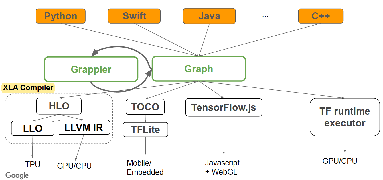
3 Graph optimization with Grappler

（原文写于 2020-05-12）

Grappler is the default graph optimization system in the TF runtime to:

• Automatically improve TF performance through graph simplifications & high-level optimizations
• Reduce device peak memory usage to enable larger models to run
• Improve hardware utilization by optimizing the mapping of graph nodes to compute resources

3.1 MetaOptimizer

Top-level driver invoked by runtime or standalone tool. Runs multiple sub-optimizers in a loop (* = not on by default):

1
2
3
4
5
6
7
8
9
10
11
12
13
14
15
16
17
18
19
20

i = 0
while i < config.meta_optimizer_iterations (default=2):
	Pruning() # Remove nodes not in fanin of outputs, unused functions
	Function() # Function specialization & inlining, symbolic gradient inlining
	CommonSubgraphElimination() # dedup Subgraph
	DebugStripper ()* # Remove assert, print, check_numerics
	ConstFold () # Constant folding and materialization
	Shape() # Symbolic shape arithmetic
	AutoMixedPrecision() # Converts data types to float16 where applicable to improve performance
	PinToHost()* # Swaps small operations onto the CPU
	Arithmetic() # Node deduping (CSE) & arithmetic simplification
	if i==0: Layout() # Layout optimization for GPU
	Remapper() # Op fusion
	Loop() # Loop Invariant Node Motion*, Stack Push & Dead Node Elimination
	Dependency () # Prune/optimize control edges, NoOp/Identity node pruning
	if i==0: Memory() # Swap-out/Swap-in, Recompute*, split large nodes
	Custom() # Run registered custom optimizers (e.g. TensorRT)
	AutoParallel()* # Automatically parallelizes graphs by splitting along the batch dimension.
Scopedallocator() # must run last: reduce data movement and to consolidate some operations.
i += 1

3.2 Pruning optimizer

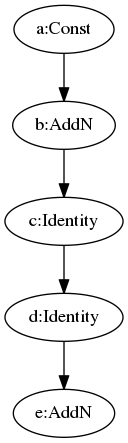
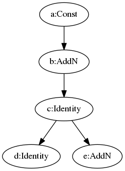
Prunes nodes that have no effect on the output from the graph. Usually run first to reduce the size of the graph and speed up other Grappler passes.

Typically removes some StopGradient and Identity nodes. For example, the Identity node below is moved to a new branch.

3.3 Function optimizer

Optimizes the function library of a TensorFlow program and inlines function bodies to enable other inter-procedural optimizations.

3.4 Common subgraph elimination

Travels the entire graph to find and dedup same subgraphs.

3.5 Debug stripper

Strips nodes related to debugging operations such as tf.debugging.Assert, tf.debugging.check_numerics, and tf.print.

OFF by default.

3.6 Constant folding optimizer

Statically infers the value of tensors when possible by folding constant nodes in the graph and materializes the result using constants.

Three methods: MaterializeShapes, FoldGraph, SimplifyGraph.

MaterializeShapes handles three nodes: Shape, Size, Rank. Because they depend only on the shape of the input tensor (not the value), MaterializeShapes replaces these three nodes with Const nodes.

FoldGraph folds nodes whose all inputs are Const — output can be pre-computed.

SimplifyGraph handles:

• Constant push-down:
• Add(c1, Add(x, c2)) => Add(x, c1 + c2)
• ConvND(c1 * x, c2) => ConvND(x, c1 * c2)
• Partial constfold:
• AddN(c1, x, c2, y) => AddN(c1 + c2, x, y),
• Concat([x, c1, c2, y]) = Concat([x, Concat([c1, c2]), y)
• Operations with neutral & absorbing elements:
• x * Ones(s) => Identity(x), if shape(x) == output_shape
• x * Ones(s) => BroadcastTo(x, Shape(s)), if shape(s) == output_shape
• Same for x + Zeros(s), x / Ones(s), x * Zeros(s) etc.
• Zeros(s) - y => Neg(y), if shape(y) == output_shape
• Ones(s) / y => Recip(y) if shape(y) == output_shape

3.7 Shape optimizer

Optimizes subgraphs that operate on shape and shape-related information.

3.8 Auto mixed precision optimizer

Converts data types to float16 where applicable to improve performance. Currently applies only to GPUs.

3.9 Pin to host optimizer

Swaps small operations onto the CPU. OFF by default.

3.10 Arithmetic optimizer

Simplifies arithmetic operations by eliminating common subexpressions and simplifying arithmetic statements.

• Arithmetic simplifications
• Flattening: a+b+c+d => AddN(a, b, c, d)
• Hoisting: AddN(x * a, b * x, x * c) => x * AddN(a+b+c)
• Simplification to reduce number of nodes:
  • Numeric: x+x+x => 3*x
  • Logic: !(x > y) => x <= y
• Broadcast minimization
• Example: (matrix1 + scalar1) + (matrix2 + scalar2) => (matrix1 + matrix2) + (scalar1 + scalar2)
• Better use of intrinsics
• Matmul(Transpose(x), y) => Matmul(x, y, transpose_x=True)
• Remove redundant ops or op pairs
• Transpose(Transpose(x, perm), inverse_perm)
• BitCast(BitCast(x, dtype1), dtype2) => BitCast(x, dtype2)
• Pairs of elementwise involutions f(f(x)) => x (Neg, Conj, Reciprocal, LogicalNot)
• Repeated Idempotent ops f(f(x)) => f(x) (DeepCopy, Identity, CheckNumerics…)
• Hoist chains of unary ops at Concat/Split/SplitV
• Concat([Exp(Cos(x)), Exp(Cos(y)), Exp(Cos(z))]) => Exp(Cos(Concat([x, y, z])))
• [Exp(Cos(y)) for y in Split(x)] => Split(Exp(Cos(x), num_splits)

3.11 Layout optimizer

Optimizes tensor layouts to execute data-format-dependent operations such as convolutions more efficiently.

For nodes including AvgPool, Conv2D, etc., they support two input formats: NHWC and NCHW. At the GPU runtime kernel, NCHW is more efficient. This optimizer adds nodes to transfer the data format before these nodes.

Original graph with all ops in NHWC format: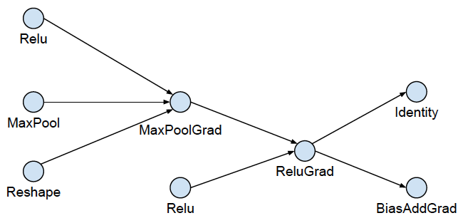

Phase 1, expand by inserting conversion pairs: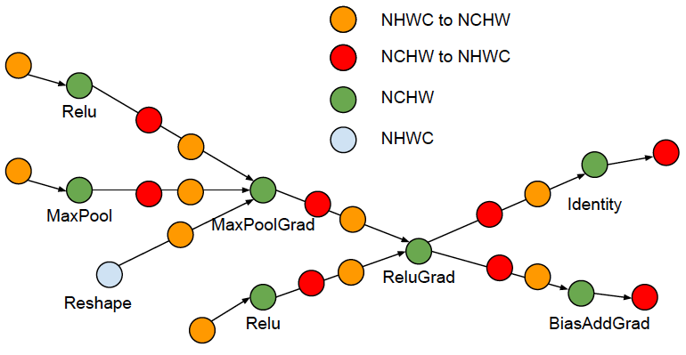

Phase 2, collapse adjacent conversion pairs: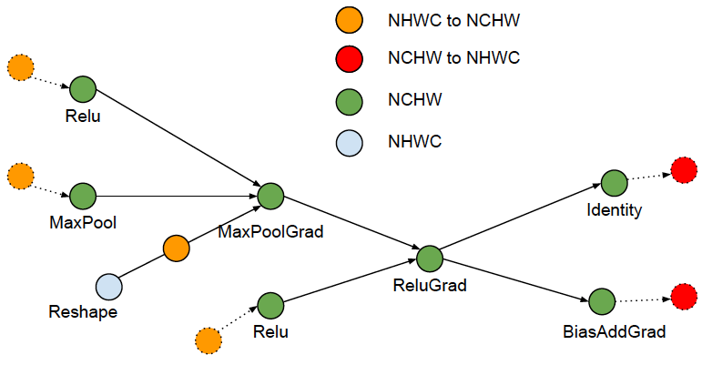

Only runs at the first iteration.

3.12 Remapper optimizer

Remaps subgraphs onto more efficient implementations by replacing commonly occurring subgraphs with optimized fused monolithic kernels:

• Conv2D + BiasAdd + <Activation>
• Conv2D + FusedBatchNorm + <Activation>
• Conv2D + Squeeze + BiasAdd
• MatMul + BiasAdd + <Activation>

Performance advantages:

• Completely eliminates Op scheduling overhead
• Improves temporal and spatial locality of data access
• E.g. MatMul is computed block-wise and bias and activation function can be applied while data is still “hot” in cache

3.13 Loop optimizer

Optimizes the graph control flow by hoisting loop-invariant subgraphs out of loops and by removing redundant stack operations in loops. Also optimizes loops with statically known trip counts and removes statically known dead branches in conditionals.

• Loop Invariant Node Motion

  1 2 3 4 5 6 7 8 9 10

  for (int i = 0; i < n; i++) { x = y + z; a[i] = 6 * i + x * x; } // Motion the y+z and x*x x = y + z; t1 = x * x; for (int i = 0; i < n; i++) { a[i] = 6 * i + t1; }

• StackPush removal
• Remove StackPushes without consumers
• Dead Branch Elimination
• Deduce loop trip count statically
• Remove loop for zero trip count
• Remove control flow nodes for trip count == 1

3.14 Dependency optimizer

Removes or rearranges control dependencies to shorten the critical path for a model step or to enable other optimizations. Also removes nodes that are effectively no-ops such as Identity.

A control edge is redundant iff there exists a path of length > 1 from source to control target: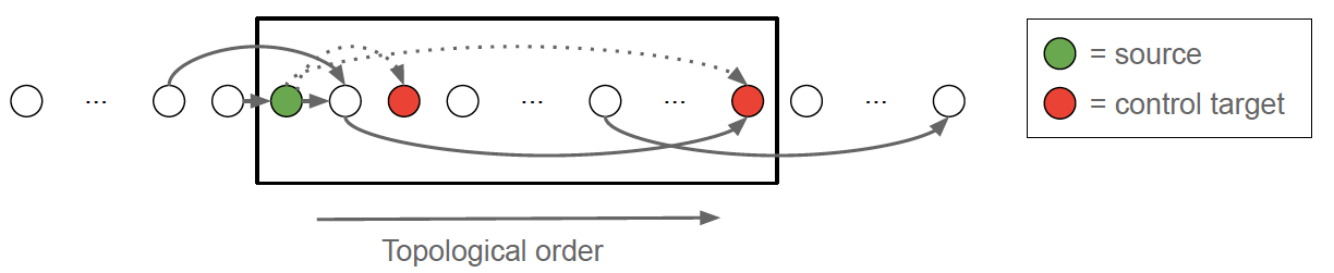

3.15 Memory optimizer

Analyzes the graph to inspect the peak memory usage for each operation and inserts CPU-GPU memory copy operations for swapping GPU memory to CPU to reduce the peak memory usage.

Memory optimization based on abstract interpretation:

• Swap-out / Swap-in optimization
• Reduces device memory usage by swapping to host memory
• Uses memory cost model to estimate peak memory
• Uses op cost model to schedule Swap-In at (roughly) the right time
• Recomputation optimization (not on by default)

Peak Memory Characterization: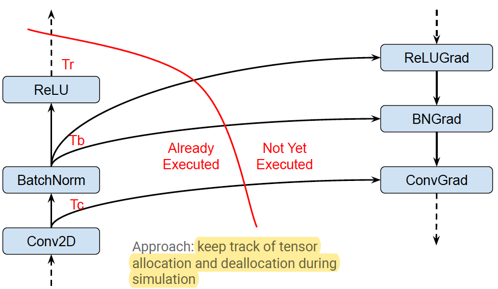

Swapping (start early):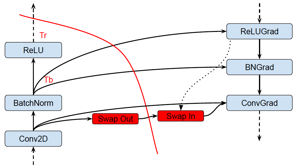

Recomputation: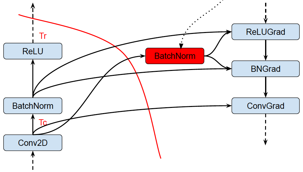

Only runs at the first iteration.

3.16 Autoparallel optimizer

Automatically parallelizes graphs by splitting along the batch dimension.

AutoParallel is similar to MirroredStrategy, but it implements parallel training by modifying the graph instead of using replicated multiple models.

For example, the following graph shows a graph where the Dequeue node fetches some samples from the FIFO node, adds with the Const node and is the input of the ApplyGradient node whose logic is var −= add * learning_rate.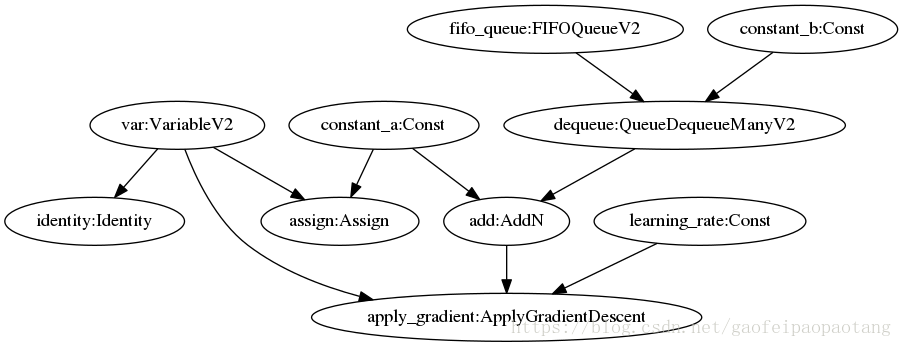

After applying AutoParallel with Replica=2, some nodes stay the same (FIFO), some are duplicated (add, Dequeue), and some new nodes are added (Div).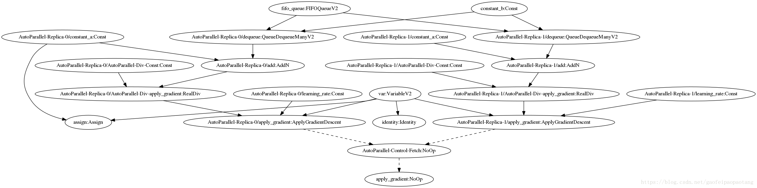

These two ApplyGradientDescent nodes can run in parallel:

var −= add(replica−0)/2 * learning_rate(replica−0)

var −= add(replica−1)/2 * learning_rate(replica−1)

OFF by default.

3.17 Scoped allocator optimizer

Introduces scoped allocators to reduce data movement and consolidate some operations. Only runs at the last iteration.

Reference

1. https://www.oreilly.com/content/distributed-tensorflow/
2. https://www.tensorflow.org/guide/distributed_training
3. https://www.tensorflow.org/guide/graph_optimization
4. https://web.stanford.edu/class/cs245/slides/TFGraphOptimizationsStanford.pdf
5. Abadi, M., Agarwal, A., Barham, P., Brevdo, E., Chen, Z., Citro, C., … & Ghemawat, S. (2016). Tensorflow: Large-scale machine learning on heterogeneous distributed systems. arXiv preprint arXiv:1603.04467.
6. Sergeev, A., & Del Balso, M. (2018). Horovod: fast and easy distributed deep learning in TensorFlow. arXiv preprint arXiv:1802.05799.
7. Abadi, M., Barham, P., Chen, J., Chen, Z., Davis, A., Dean, J., … & Kudlur, M. (2016). Tensorflow: A system for large-scale machine learning. In 12th {USENIX} Symposium on Operating Systems Design and Implementation ({OSDI} 16) (pp. 265-283).
8. Mirhoseini, A., Pham, H., Le, Q. V., Steiner, B., Larsen, R., Zhou, Y., … & Dean, J. (2017, August). Device placement optimization with reinforcement learning. In Proceedings of the 34th International Conference on Machine Learning-Volume 70 (pp. 2430-2439). JMLR. org.
9. https://leimao.github.io/blog/Data-Parallelism-vs-Model-Paralelism/
10. Goyal, P., Dollár, P., Girshick, R., Noordhuis, P., Wesolowski, L., Kyrola, A., … & He, K. (2017). Accurate, large minibatch sgd: Training imagenet in 1 hour. arXiv preprint arXiv:1706.02677.
11. https://github.com/tensorflow/tensorflow/blob/master/tensorflow/core/grappler/optimizers/meta_optimizer.cc